dplyr

Set up

How to open a saved Rproj and read in data if not already open

Open your saved Rproj in Rstudio by clicking File menu then Open project and look for your .Rproj file. Click the Files tab in the bottom right pane, click the data folder and check the penguins.csv is in there. Then read it in.

penguins <- read.csv(file = "data/penguins.csv")

1 Data wrangling

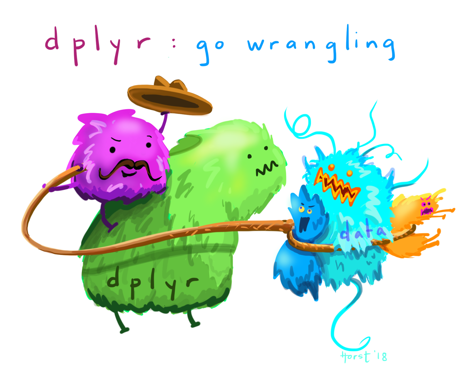Artwork by @allison_horst

Cleaning or wrangling data means many things to many researchers: we often select certain observations (rows) or variables (columns), we often group the data by a certain variable(s), or we even calculate summary statistics. We can do these operations using the normal base R functions:

mean(penguins[penguins$species == "Adelie", "body_mass_g"], na.rm = TRUE)
mean(penguins[penguins$species == "Gentoo", "body_mass_g"], na.rm = TRUE)
mean(penguins[penguins$species == "Chinstrap", "body_mass_g"])

But this isn’t very nice because there is a fair bit of repetition. Repeating yourself will cost you time, both now and later, and potentially introduce some nasty bugs.

1.1 The dplyr package

Luckily, the dplyr package provides a number of very useful functions for manipulating dataframes in a way that will reduce the above repetition, reduce the probability of making errors, and save you some typing. As an added bonus, you might even find the dplyr grammar easier to understand.

Here we’re going to cover 5 of the most commonly used functions as well as using pipes (%>%) to combine them.

1. select()
2. filter()
3. group_by()
4. summarize()
5. mutate()

If you have not installed this package previously, use the packages tab, bottom right.

Then load the package:

library("dplyr")

1.2 select()

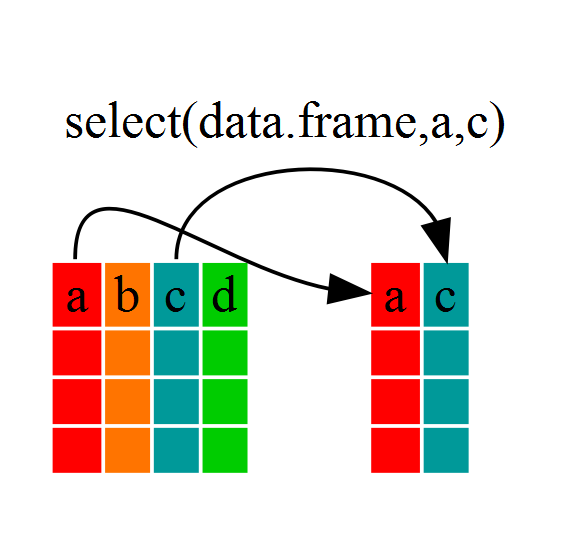
If we wanted to analyse only a few of the variables (columns) in our dataframe we could use the select() function. This will keep only the variables you select.

species_body <- select(penguins, species,body_mass_g,sex)

If we open up species_body (under the environment tab) we’ll see that it only contains the species, body mass and sex.

1.3 filter()

If we now wanted to use the columns selected above, but only with Adelie penguins, we can use filter

species_body_adelie <- filter(species_body, species =="Adelie")

Open species_body_adelie to check it only contains Adelie penguin data.

Above we used ‘normal’ grammar, but the strengths of dplyr lie in combining several functions using pipes.

To demonstrate a pipe (%>%) let’s repeat what we’ve done above by combining select and filter in one command.

species_body_adelie2 <- penguins %>%
    filter(species == "Adelie") %>%
    select(species, body_mass_g, sex)

First we assign the result to species_body_adelie2. Then, we call the penguins dataframe and pass it on, using the pipe symbol %>% to the filter() function. We don’t need to name which data object to use in the filter() function since we’ve piped penguins in. Then the resulting data frame is piped into the select() part of the code.

Pipes allow you to do many actions in one command, make code easier to read and avoid creating multiple data objects.

Challenge 1

Write a single command (which spans multiple lines and include pipes) that will produce a dataframe that has the Gentoo values for island, flipper_length_mm and year, but not for other penguins. How many rows does your dataframe have?

Check your answer to Challenge 1

You should have 124 rows (look in the environment tab in the top right window to check this).

Note: The order of operations is very important in this case. If we used ‘select’ first, filter would not be able to find the variable species since we would have removed it in the previous step

1.4 group_by() and summarize()

If we want to do the above for each species, we’d have to repeat the code but we’re trying to reduce the error prone repetitiveness of what can be done with base R. In other words, using filter(), will only pass observations that meet your criteria (in the above: species=="Adelie"). Instead, we can use group_by(), which will analyse all three species.

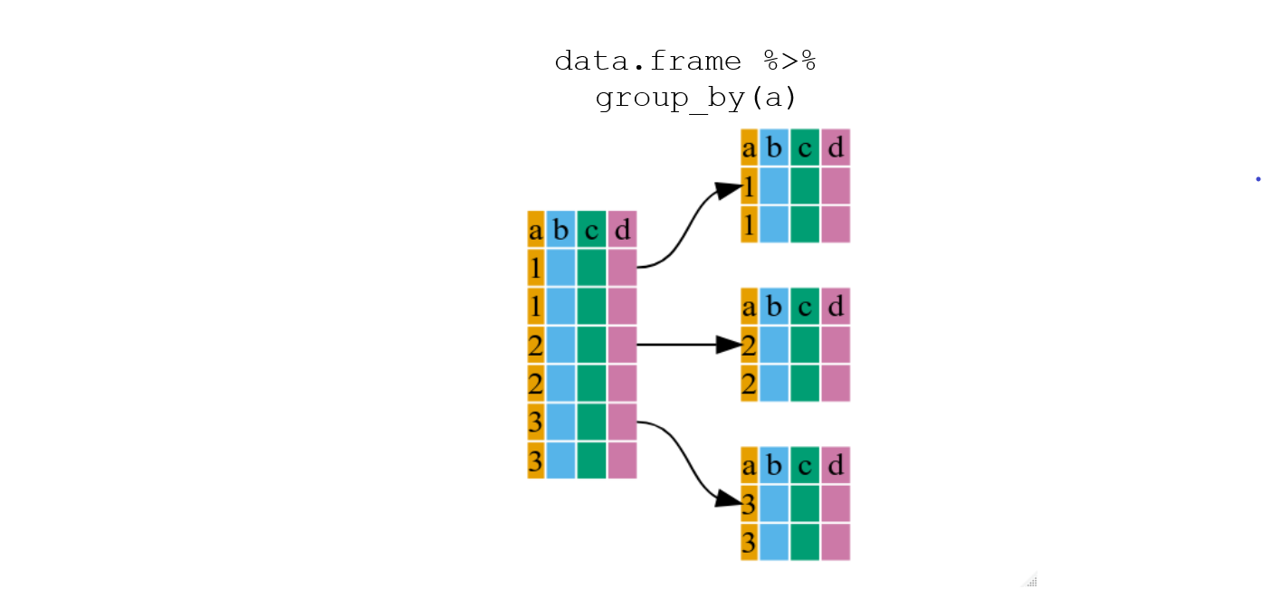
1.4.1 Using group_by() with summarize()

group_by() is more easily understood when it’s used with something like summarize(). By using the group_by() function, we split our original data frame into multiple pieces, then we can run functions (e.g. mean() or sd()) within summarize().

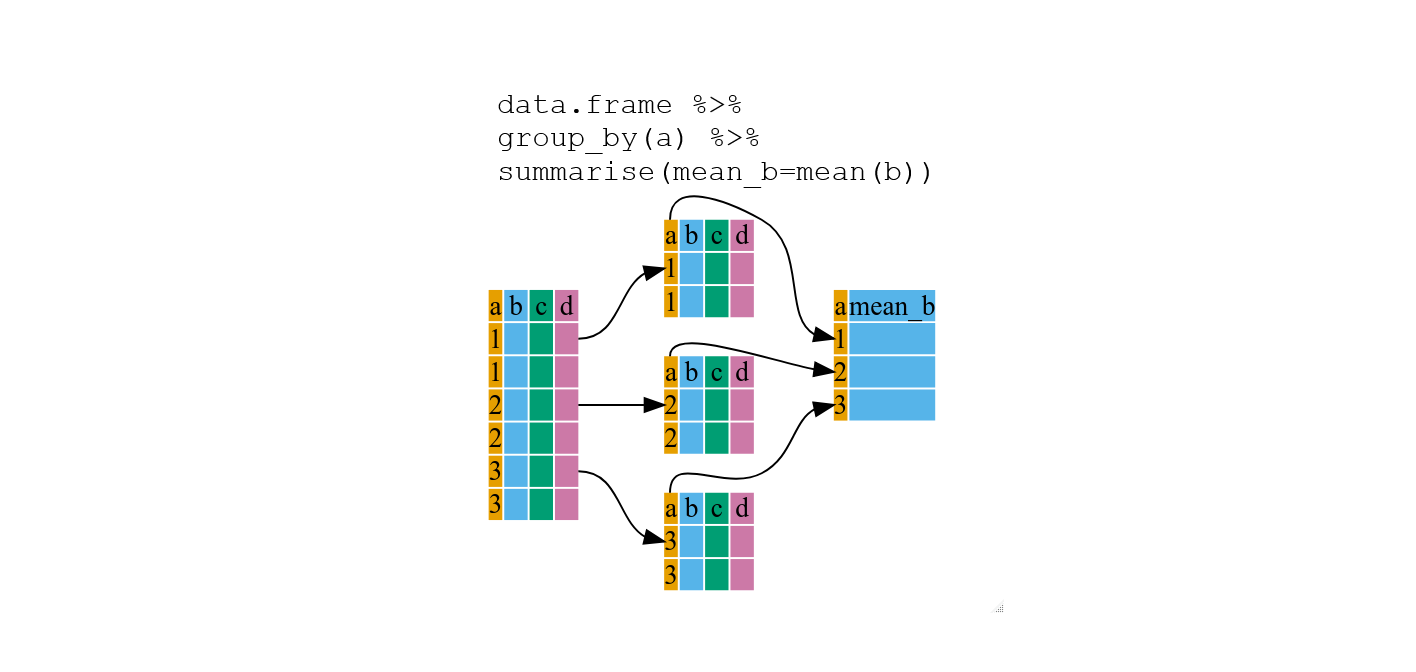
penguins %>%
    group_by(species) %>%
    summarize(mean_body = mean(body_mass_g, na.rm=TRUE))

## # A tibble: 3 × 2
##   species   mean_body
##   <chr>         <dbl>
## 1 Adelie        3701.
## 2 Chinstrap     3733.
## 3 Gentoo        5076.

Tip: To assign or not

Starting the code with species_body_means <- will assign the results as a new data frame called species_body_means. This species_body_means will then be listed under the environment tab so you can view it. Good for large results data frames.

As was done in the last example, you can choose not to assign as an object if the resulting data frame is small. The results are not saved but given in your console window.

The function group_by() allows us to group by multiple variables. Let’s group by species and sex.

penguins %>%
    group_by(species, sex) %>%
    summarize(mean_body = mean(body_mass_g, na.rm=TRUE))

And you’re not limited to analysing only one variable with only one function in summarize().

penguins %>%
    group_by(species, sex) %>%
    summarize(mean_body = mean(body_mass_g),
              sd_body = sd(body_mass_g),
              mean_flipper = mean(flipper_length_mm),
              sd_flipper = sd(flipper_length_mm))

The filter() function can remove the penguins who have NA under sex. (Read the exclamation mark as “not”)

penguins %>%
    group_by(species, sex) %>%
    filter(!is.na(sex)) %>%
    summarize(mean_body = mean(body_mass_g),
              sd_body = sd(body_mass_g),
              mean_flipper = mean(flipper_length_mm),
              sd_flipper = sd(flipper_length_mm))

Challenge 2

For each species and sex, calculate the mean and sd of bill length and bill depth.

Exporting such information as a journal style table is useful as it can be added to Word documents for assessments.

Challenge 3

Write code that takes the table you created in Challenge 2, formats it using gt() function and exports it as a html file using gtsave(), saving it in your results folder. The table should look like the below.

Species	Sex	Mean Bill Length	SD Bill Length	Mean Bill Depth	SD Bill Depth
Adelie	female	37.25753	2.028883	17.62192	0.9429927
Adelie	male	40.39041	2.277131	19.07260	1.0188856
Chinstrap	female	46.57353	3.108669	17.58824	0.7811277
Chinstrap	male	51.09412	1.564558	19.25294	0.7612730
Gentoo	female	45.56379	2.051247	14.23793	0.5402493
Gentoo	male	49.47377	2.720594	15.71803	0.7410596

Solution to Challenge 2 and 3

Create a summary table

penguinSummary <- penguins %>%
  group_by(species, sex) %>%
  filter(!is.na(sex)) %>%
  summarize(
    mean_billlength = mean(bill_length_mm),
    sd_billlength = sd(bill_length_mm),
    mean_billdepth = mean(bill_depth_mm),
    sd_billdepth = sd(bill_depth_mm),
    .groups = "drop"  
  )

formatted_table <- penguinSummary %>%
  gt() %>%
  cols_label(
    species = "Species",
    sex = "Sex",
    mean_billlength = "Mean Bill Length",
    sd_billlength = "SD Bill Length",
    mean_billdepth = "Mean Bill Depth",
    sd_billdepth = "SD Bill Depth"
  ) %>%
  tab_options(column_labels.border.top.color = "black",
  column_labels.border.bottom.color = "black",
  table_body.border.bottom.style = "none",
  table.border.bottom.color = "black",
  table_body.hlines.style = "none")

Format the table

formatted_table <- penguinSummary %>%
  gt() %>%
  cols_label(
    species = "Species",
    sex = "Sex",
    mean_billlength = "Mean Bill Length",
    sd_billlength = "SD Bill Length",
    mean_billdepth = "Mean Bill Depth",
    sd_billdepth = "SD Bill Depth"
  ) %>%
  tab_options(column_labels.border.top.color = "black",
  column_labels.border.bottom.color = "black",
  table_body.border.bottom.style = "none",
  table.border.bottom.color = "black",
  table_body.hlines.style = "none")

Save the table

gtsave(formatted_table, "results/penguin_summary_table.html")

1.5 count() and n()

If we wanted to check the number of penguins included in the dataset for the year 2007, we can use filter() then the count() function:

penguins %>%
    filter(year == 2007) %>%
    count

If we need to use the total number of observations in calculations, the n() function is useful. For instance, if we wanted the standard error of body mass per species:

penguins %>%
    group_by(species) %>%
    summarize(se_body = sd(body_mass_g)/sqrt(n()))

This works better if we filter out the NAs.

penguins %>%
    group_by(species) %>%
    filter(!is.na(body_mass_g)) %>%
    summarize(se_body = sd(body_mass_g)/sqrt(n()))

Tip: Standard error

To calculate standard error (se), the standard deviation (sd) is divided by the square root of the sample size (n). \(se = sd/\sqrt n\)

1.6 mutate()

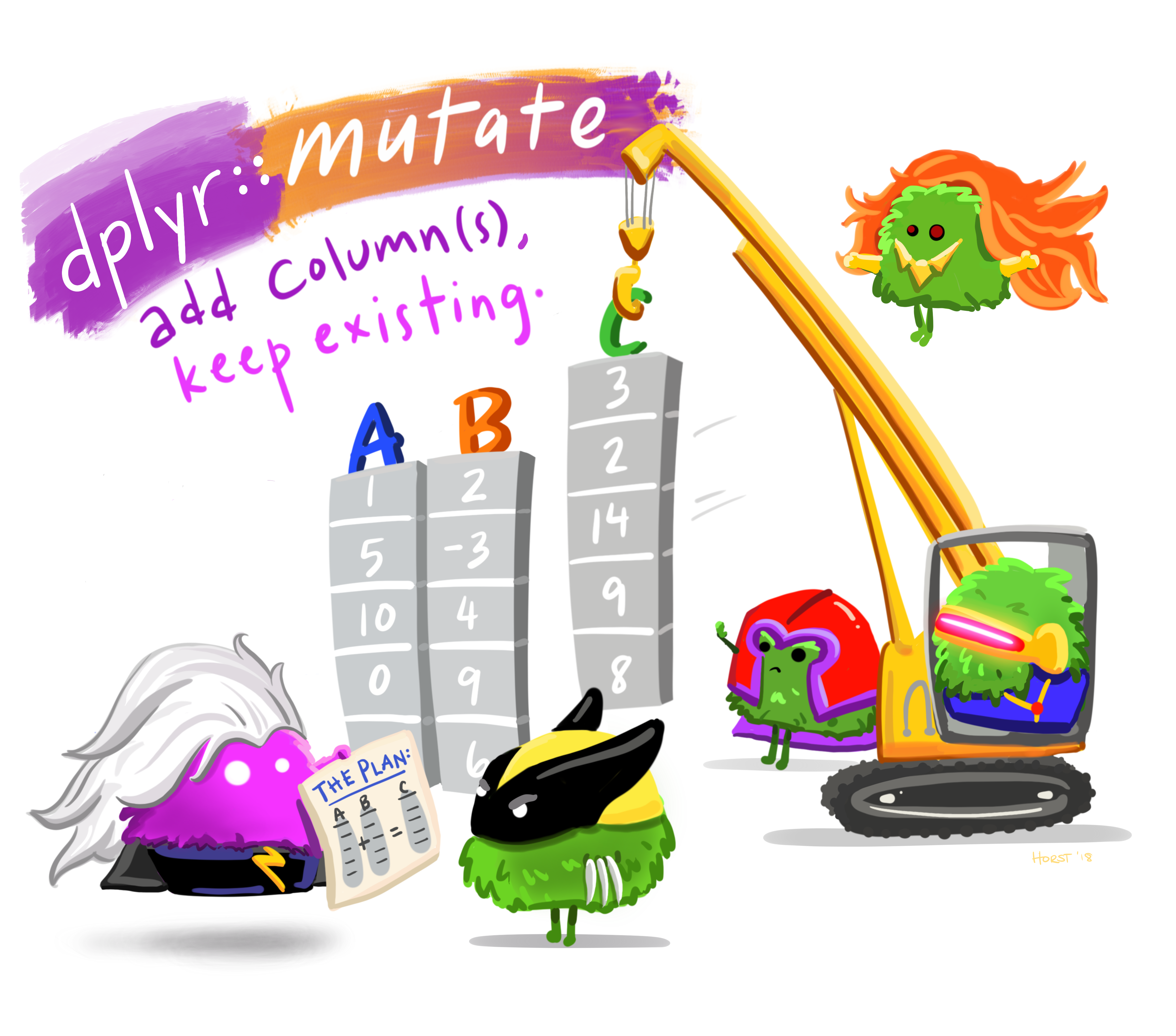Artwork by @allison_horst

mutate() creates new variables (columns) from existing variables.

penguins_body_kg <- penguins %>%
    mutate(body_weight_kg = body_mass_g / 1000)

1.6.1 Connect mutate with case_when

We can combine mutate() with case_when() to filter data in the moment of creating a new variable. (Note: case_when() is an alternative to the older ifelse() function.)

We can make a new column of data that categorises each Gentoo penguin as either large or small and all other penguins as “not Gentoo”. To do this, we use information in the species and body mass columns.

penguin_gentoo_bodysize <- penguins %>%
  mutate(
    size = case_when(
      species == "Gentoo" & body_mass_g >= 5000 ~ "large",
      species == "Gentoo" & body_mass_g < 5000 ~ "small",
      TRUE ~ "not Gentoo"
                    )
        )

Size is our name for the new column. You can read ~ as “then write”. The last line of code can be read as “if none of the conditions are TRUE then write not Gentoo”.

Advanced Challenge

Write code to select only the species, island, flipper length and sex variables. Filter to only the Adelie penguins. Filter out the penguins with NA under flipper length. Group the data by island. Use mutate to create a new flipper length column in cm by dividing the flipper length by 100. Summarise the mean and sd of flipper lengths for each of the islands.

Solution to Advanced Challenge

penguins %>%
    select(species, island, flipper_length_mm, sex) %>%
    filter(species == "Adelie") %>%
    filter(!is.na(flipper_length_mm)) %>%
    group_by(island) %>%
    mutate(flipper_cm = flipper_length_mm/100) %>%
    summarise(flipper_mean_cm = mean(flipper_cm),
              flipper_sd = sd(flipper_cm))

## # A tibble: 3 × 3
##   island    flipper_mean_cm flipper_sd
##   <chr>               <dbl>      <dbl>
## 1 Biscoe               1.89     0.0673
## 2 Dream                1.90     0.0659
## 3 Torgersen            1.91     0.0623

1.7 Handling missing values

If there are blank cells in the file you read into R, it will fill them in with NA.

We have seen that some functions use the NA remove argument to deal with NA values, as below.

mean(penguins[penguins$species == "Adelie", "body_mass_g"], na.rm = TRUE)

The filter function used !is.na read as “not is NA”.

penguins %>%
    group_by(species, sex) %>%
    filter(!is.na(sex))

An alternative is using na.omit()

clean_data <- na.omit(penguins)

Caution!

Be aware thatna.omit() removes the entire row of data even if there is an NA value in a variable you are not using.

If missing values are coded as an extreme value such as 999, you must change them to NA.

ExampleData[ExampleData == 999] <- NA

Tip: missing values

Be careful using 0. Zero should mean the measurement was 0 units oppose to missing data.

1.8 Other great resources

• R for Data Science
• Data Wrangling Cheat Sheet
• Introduction to dplyr
• Data wrangling with R and RStudio

Source

Adapted from R for Reproducible Scientific Analysis licensed CC_BY 4.0 by The Carpentries