tidyr

set up

To use the tidyr package you will need to ensure you have it installed on the computer you are using (hint: use the Packages tab, bottom right) and then load it.

library(tidyr)

1 Tidy Data

The same data can be laid out in a spreadsheet in a number of different ways.

“Tidy” data has a layout that makes it easier to do analyses in R. Real data is rarely in the format you need for analysis and often needs to be changed.

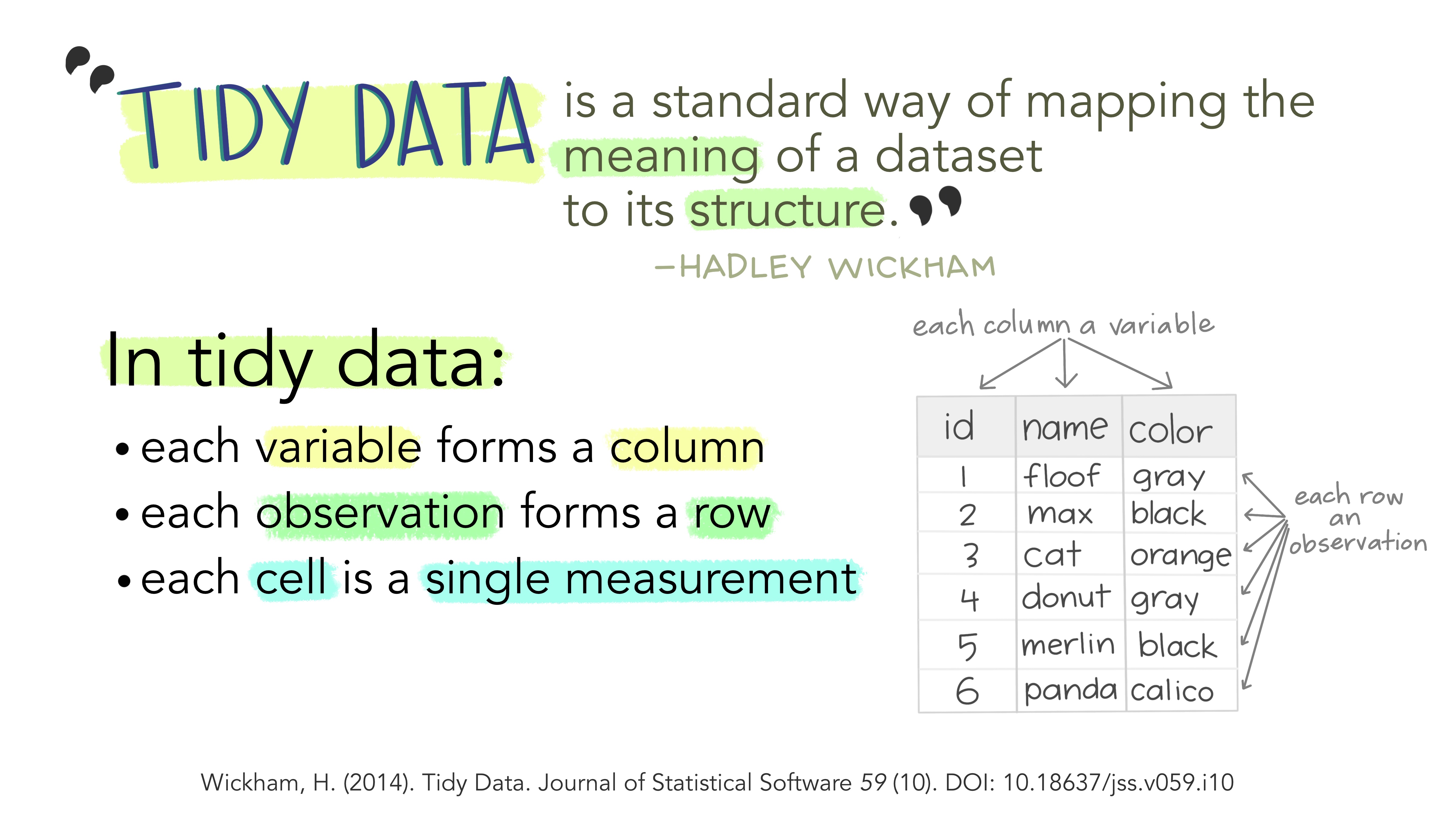Artwork by @allison_horst

1.1 Examples

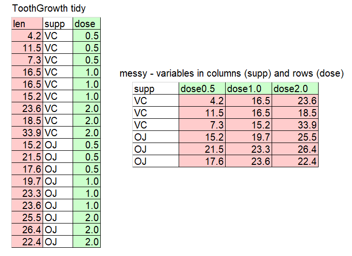
Study the cartoon and the tables to understand what tidy data is.

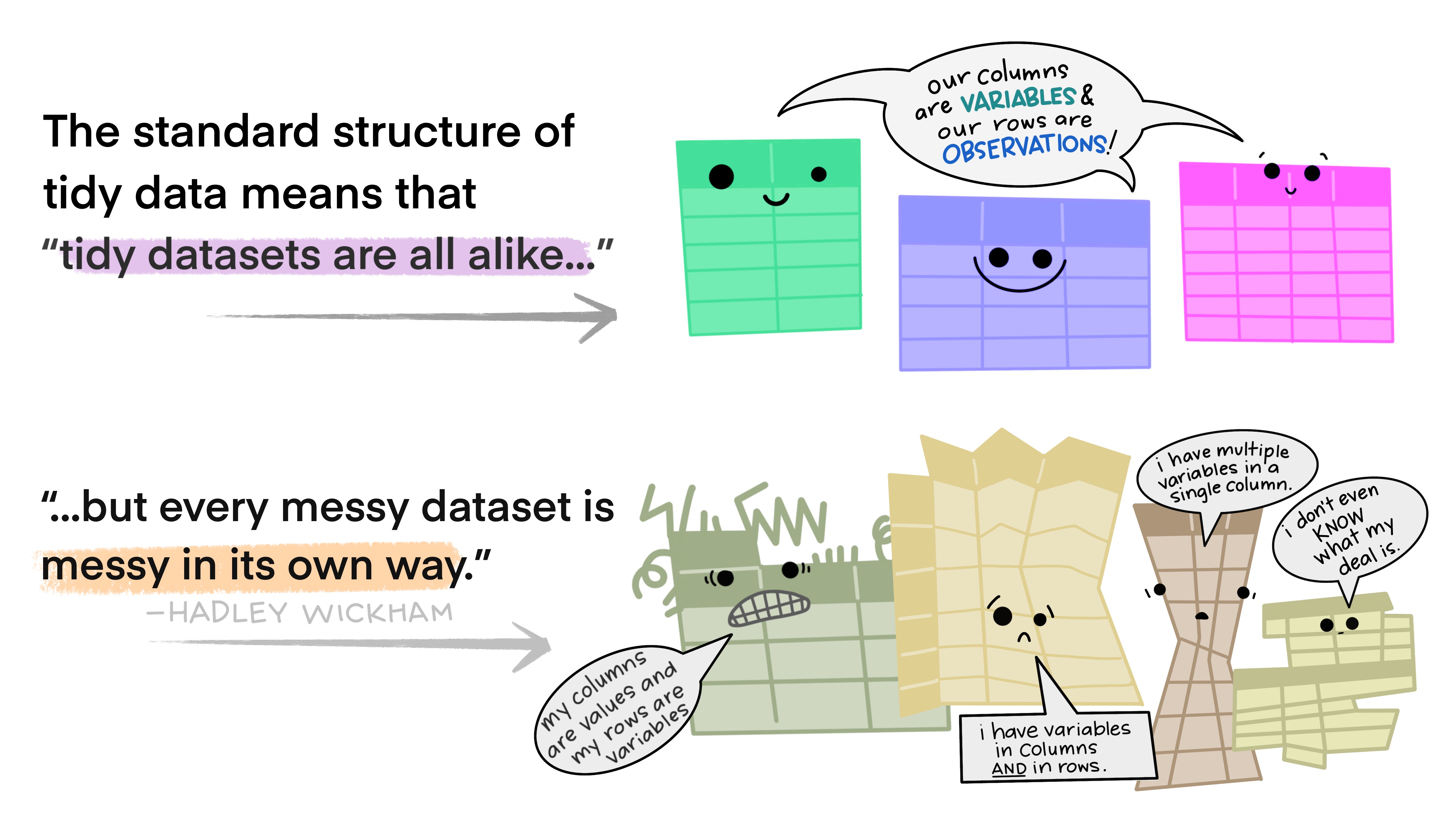
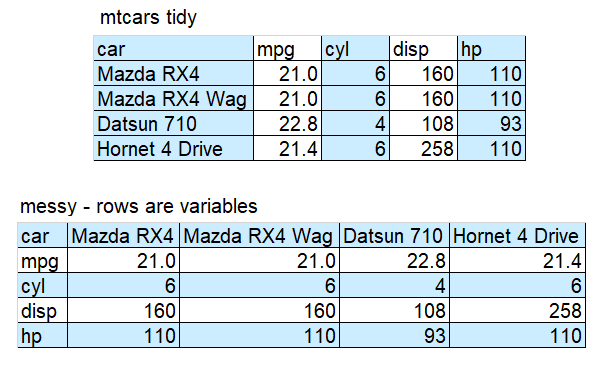
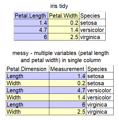
Tip: Example data

This data is sampled from datasets (mtcars, iris, ToothGrowth) commonly used on R internet help forums. Being familiar with the column names helps you to understand where the variables should go when you adapt example code.

Challenge 1

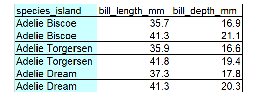
Decide if this data is tidy or messy. Explain why.

Solution to Challenge 1

The data is messy because there are two variables (species and island) in a single column. In other words, there are two observations in each of the cells in the first column. The corresponding tidy version is below.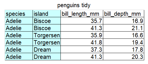

1.2 separate()

Since “…every messy dataset is messy in it’s own way” there are many functions you might need to change data. separate() is just one example.

To demonstrate separate() we will first create the messy data set in the Challenge above using the combine c() function. (In internet help forums you may see small example data frames (df) created in this way.)

penguin_messy_df <- data.frame(
  species_island = c(rep("Adelie Biscoe", 2), rep("Adelie Torgersen", 2), rep("Adelie Cream", 2)), # `rep()` is the repeat function. 
  bill_length_mm = c(35.7, 41.3, 35.9, 41.8, 37.3, 41.3),
  bill_depth_mm = c(16.9, 21.1, 16.6, 19.4, 17.8, 20.3)
)

If you run this code for yourself you can view the data frame under the environment tab.

Now we can use separate() to split the species_island column into two columns and create a new data frame called penguin_tidy_df.

penguin_tidy_df <- separate(
  penguin_messy_df, # the data frame we want to change
  col = species_island, # the column we want separated
  into = c('species', 'island'), # the names of the new columns we want to create
  sep = ' ') # what separates the data. In our case a space

View penguin_tidy_df to make sure it’s worked.

1.3 long and wide data

Another way you may need to change data is by making it “longer” or “wider” using the functions pivot_longer() and pivot_wider(). Study the examples in the following sections so you understand the difference between the two data formats.

1.3.1 pivot_wider

This code creates a small data frame in long format:

population_long <- data.frame(
  country = c(rep("Chad", 2), rep("Cuba", 2), rep("Fiji", 2), rep("Iran", 2)),
  year = rep(c(2000, 2020), 4),
  population = c(9755000, 16818391, 11269000, 11113215, 848000, 898402, 69515000, 85655490)
)
population_long

##   country year population
## 1    Chad 2000    9755000
## 2    Chad 2020   16818391
## 3    Cuba 2000   11269000
## 4    Cuba 2020   11113215
## 5    Fiji 2000     848000
## 6    Fiji 2020     898402
## 7    Iran 2000   69515000
## 8    Iran 2020   85655490

The function pivot_wider() is used to make each year a new column, with the values under population used to fill the new columns:

population_wide <- pivot_wider(
  population_long, # the data frame to be made wider
  names_from = year, # the column to take the names for the new columns from
  values_from = population, # the column to take values from to fill in the new columns
                               )
population_wide

## # A tibble: 4 × 3
##   country   `2000`   `2020`
##   <chr>      <dbl>    <dbl>
## 1 Chad     9755000 16818391
## 2 Cuba    11269000 11113215
## 3 Fiji      848000   898402
## 4 Iran    69515000 85655490

1.3.2 pivot_longer

This code, which creates a small data frame in wide format, shows fish weights before and after a treatment:

fish_wide <- data.frame(
  fish = c(1:4),
  before = c(12.4, 12.9, 11.2, 10.8),
  after = c(13.1, 13.2, 12.3, 11.7)
)
fish_wide

##   fish before after
## 1    1   12.4  13.1
## 2    2   12.9  13.2
## 3    3   11.2  12.3
## 4    4   10.8  11.7

The function pivot_longer() is used to take the headings before and after and repeat in a column named time and put the measurements in a new column called weights:

fish_long <- pivot_longer(fish_wide, 
  cols = c(before, after), # columns to pivot from wide to long
  names_to = "time", # name of the new column for the categories
  values_to = "weight" # name of the new column where the values go
)
fish_long

## # A tibble: 8 × 3
##    fish time   weight
##   <int> <chr>   <dbl>
## 1     1 before   12.4
## 2     1 after    13.1
## 3     2 before   12.9
## 4     2 after    13.2
## 5     3 before   11.2
## 6     3 after    12.3
## 7     4 before   10.8
## 8     4 after    11.7

Challenge 2

Use the code to create a wide data set containing the height of four people as children and adults. Use pivot_longer to make the data long. You can reveal the Hint if you need to.

people_heights_wide <- data.frame(
  person = 1:4,
  child = c(85.4, 79.1, 81.9, 90.1),
  adult = c(170.1, 165.9, 168.8, 183.7)
)

Hint

The columns to pivot are child and adult. The name of the new column could be “age” The name of the new column for the measurements could be “height”

Solution to Challenge 2

pivot_longer(people_heights_wide, 
  cols = c(child, adult),    
  names_to = "age", 
  values_to = "height"
)

## # A tibble: 8 × 3
##   person age   height
##    <int> <chr>  <dbl>
## 1      1 child   85.4
## 2      1 adult  170. 
## 3      2 child   79.1
## 4      2 adult  166. 
## 5      3 child   81.9
## 6      3 adult  169. 
## 7      4 child   90.1
## 8      4 adult  184.

Tip: Collecting data

These are small, simple examples. Real data can be difficult to change.

If you are collecting your own data, plan in detail how the data will be analysed so that as you record data you arrange it in your spreadsheet in a way that will make data wrangling and analysis easier.

Source